Memory in Transformers (2): Associative Memory as Test-Time Regression
Instead of naively compressing the KV cache, new architectures (e.g. Mamba, RWKV, DeltaNet, Titans, etc.) differentially weigh associative memories. We can generalise these approaches as test-time regression solvers that dynamically adjust weights to reflect relevance of past information.
To recap, we showed that a KV cache can be compressed into a finite hidden state that cleanly retrieves a value, given the associated key. We can phrase this as a minimisation problem,
\[\min_{m \in \mathcal{M}} \frac{1}{2} \sum_{i=1}^t \gamma_i \,\| \mathbf{v}_i - m(k_i)\|_2^2\]where a model, $m$, learns to minimise the retrieval of a value, given a key, weighted by how important this association should be, $\gamma_i$. Here, we will see how this genralisation leads to different architectures for associative memory.
Associative Memory as Test-Time Regression
Today, everyone and their dog is releasing a new linear Transformer architecture. They mostly belong to a few families that take different approaches at the memory compression problem. Wang et al., (2025) neatly summarise how this is just test-time regression, like above, with each family adopting different regressor functions, weightings, and optimisation algorithms.
Let’s take our vanilla linear attention and show that this is just an approximation of linear least squares i.e. no $\gamma_i$, $\mathcal{M}$ restricted to being linear, and solvable analytically:
\[m_{\text{linear}} = \arg\min_{m \in \mathcal{M}} \frac{1}{2} \sum_{i=1}^t \,\| \mathbf{v}_i - m(k_i)\|_2^2 = \mathbf{V}^\top \mathbf{K} \left( \mathbf{K}^\top \mathbf{K} \right)^{-1} \scriptstyle{\mid} \, {\scriptstyle t \, > \, d_{\text{keys}}}\]Calculating $\small{\left( \mathbf{K}^\top \mathbf{K} \right)^{-1}}$ is computationally expensive, but if we assume that key embeddings are approximately orthogonal to one another, we can make the approximation $\mathbf{K}^\top \mathbf{K} = \mathbf{I}$. Notice now that we have solved $M_{\text{t}} \approx \sum_{i=1}^t \mathbf{v_i}\mathbf{k_i}^T$, which is just our compressed KV-cache. Here $\phi (\mathbf{k_i})$ is a linear kernel, but we can also use linear attention with a nonlinear feature map, which can be solved by the same approximation as above. This is essentially what The Hedgehog and DiJian do.
Unlike linear attention, gated linear attention and state-space models implement time-decayed memory updates. We can model this as weighted linear least squares,
\[m_{\text{weighted linear}} = \arg\min_{m \in \mathcal{M}} \frac{1}{2} \sum_{i=1}^t \gamma^{(t)} \,\| \mathbf{v}_i - m(k_i)\|_2^2 = \mathbf{V}^\top \boldsymbol{\Gamma} \mathbf{K} \left( \mathbf{K}^\top \boldsymbol{\Gamma} \mathbf{K} \right)^{-1} \scriptstyle{\mid} \, {\scriptstyle t \, > \, d_{\text{keys}}}\]where we geometrically decay in time, $\gamma_i^{(t)} = \prod_{j=i+1}^{t} \gamma_j$, and $\boldsymbol{\Gamma}$ is a diagonal of $\gamma_i^{(t)}$ in time. Following the orthogonality approximation before, $\mathbf{K}^\top \boldsymbol{\Gamma} \mathbf{K} \approx \mathbf{I}$, we find an approximate analytical solution, which we can state as a recurrence relationship,
\[\mathbf{M}_t \approx \sum_{i=1}^t \gamma_i^{(t)} \mathbf{v}_i \mathbf{k}_i^\top = \sum_{i=1}^t \left( \prod_{j=i+1}^t \gamma_j \right) \mathbf{v}_i \mathbf{k}_i^\top = \gamma_t \sum_{i=1}^{t-1} \gamma_i^{(t-1)} \mathbf{v}_i \mathbf{k}_i^\top + \mathbf{v}_t \mathbf{k}_t^\top = \gamma_t \mathbf{M}_{t-1} + \mathbf{v}_t \mathbf{k}_t^\top\]This looks a lot like recent state-space models (Mamba-2) and gated linear attention (GLA, RWKV-6, mLSTM).
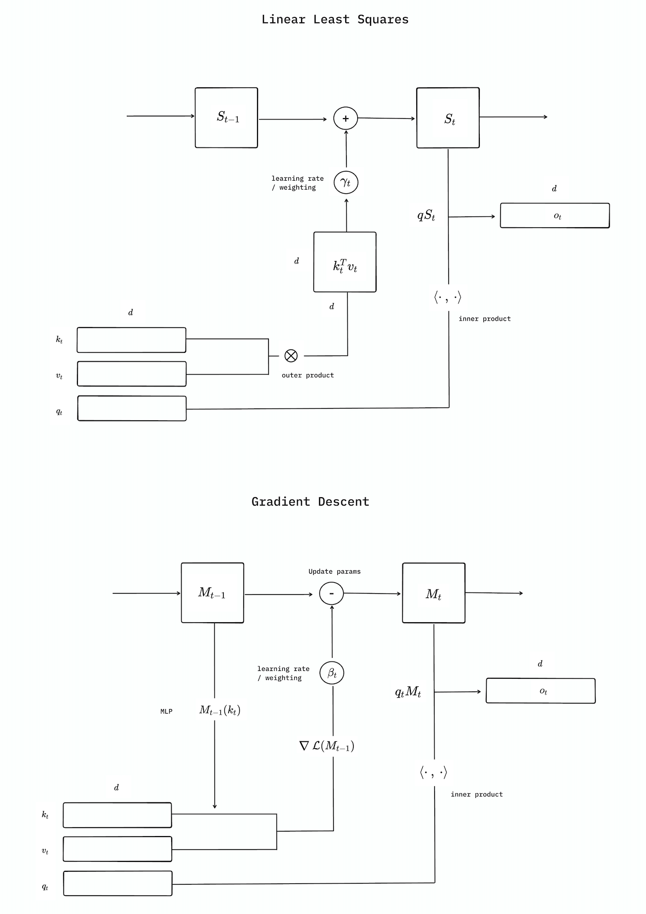
The methods above solve the regression problem analytically, via a second-order solution. In order to be computationally feasible, they approximate the solution by ignoring the inversion, which leads to poor results in practice. We can instead try a first order solution like online gradient descent, which is computationally less expensive. This looks a lot more like what Schmidhuber had in mind with online learning via fast weights. Here, our model is not longer a naively summed hidden state – it’s an MLP that learns. For SGD, this looks like,
\[\nabla \mathcal{L}_t(\mathbf{M}) = \nabla \sum_{i=1}^t \frac{1}{2} \|\mathbf{v}_i - \mathbf{M}\mathbf{k}_i\|_2^2 = (\mathbf{M}\mathbf{K}^\top - \mathbf{V}^\top)\mathbf{K}\]We can now write the recurrence relationship as,
\[\begin{align*} \mathbf{M}_t &= \mathbf{M}_{t-1} - \beta_t \nabla \mathcal{L}_t(\mathbf{M}_{t-1}) \\ &= \mathbf{M}_{t-1} + \beta_t (\mathbf{v}_t - \mathbf{M}_{t-1} \mathbf{k}_t) \mathbf{k}_t^\top \\ &= \mathbf{M}_{t-1} (\mathbf{I} - \beta_t \mathbf{k}_t \mathbf{k}_t^\top) + \beta_t \mathbf{v}_t \mathbf{k}_t^\top \end{align*}\]where $\beta_t$ is the learning rate or step-size for batched updates. The “learning to memorise at test-time” paradigm is exaclty this. It’s used by TTT and DeltaNet. Titans also uses this, but adds momentum by having two hidden states, which they show stabilises learning. Longhorn uses adaptive updates
You can now start to appreciate the immense design freedom we can have with this, beyond vanilla SGD. Some ideas Wang et al., (2025) proposed include adaptive
Again, we see that we just generate an online sequence of associative memories that can map our keys back to our values. The diagram below shows how the online-learning method differs from recursive least squares,