The Blessings of Dimensionality

Understanding spaces in high dimensions is surprisingly unintuitive. A simple example that illustrates this is scaling a sphere to infinite dimensions, where its volume tends to zero.

Let’s show this mathematically. The volume of a sphere is given by:

\[V_n(r) = \frac{\pi^{n/2}}{\Gamma(n/2 + 1)} r^n\]

If you have seen this equation before, we have a straighforward proof that the volume tends to zero.

$$ V_n(1) \,=\, \frac{\pi^{\frac{n}{2}}}{\Gamma\!\Bigl(\frac{n}{2}+1\Bigr)} \;\overset{\text{Stirling}}{\sim}\; \frac{\pi^{\frac{n}{2}}}{ \sqrt{\pi n}\,\Bigl(\tfrac{n}{2e}\Bigr)^{\frac{n}{2}} } \;=\; \frac{1}{\sqrt{\pi n}} \left(\frac{2e\pi}{n}\right)^{\!\tfrac{n}{2}} \;\xrightarrow[n\to\infty]{}\;0 $$ To simplify notation, this considers a unit sphere, $r=1$.

Unfortunately it’s a little difficult to develop an intuition around this formula. A nicer way to visualise this is to think of a ball (by which I mean a hypersphere) as a stack of discs in a lower dimension.

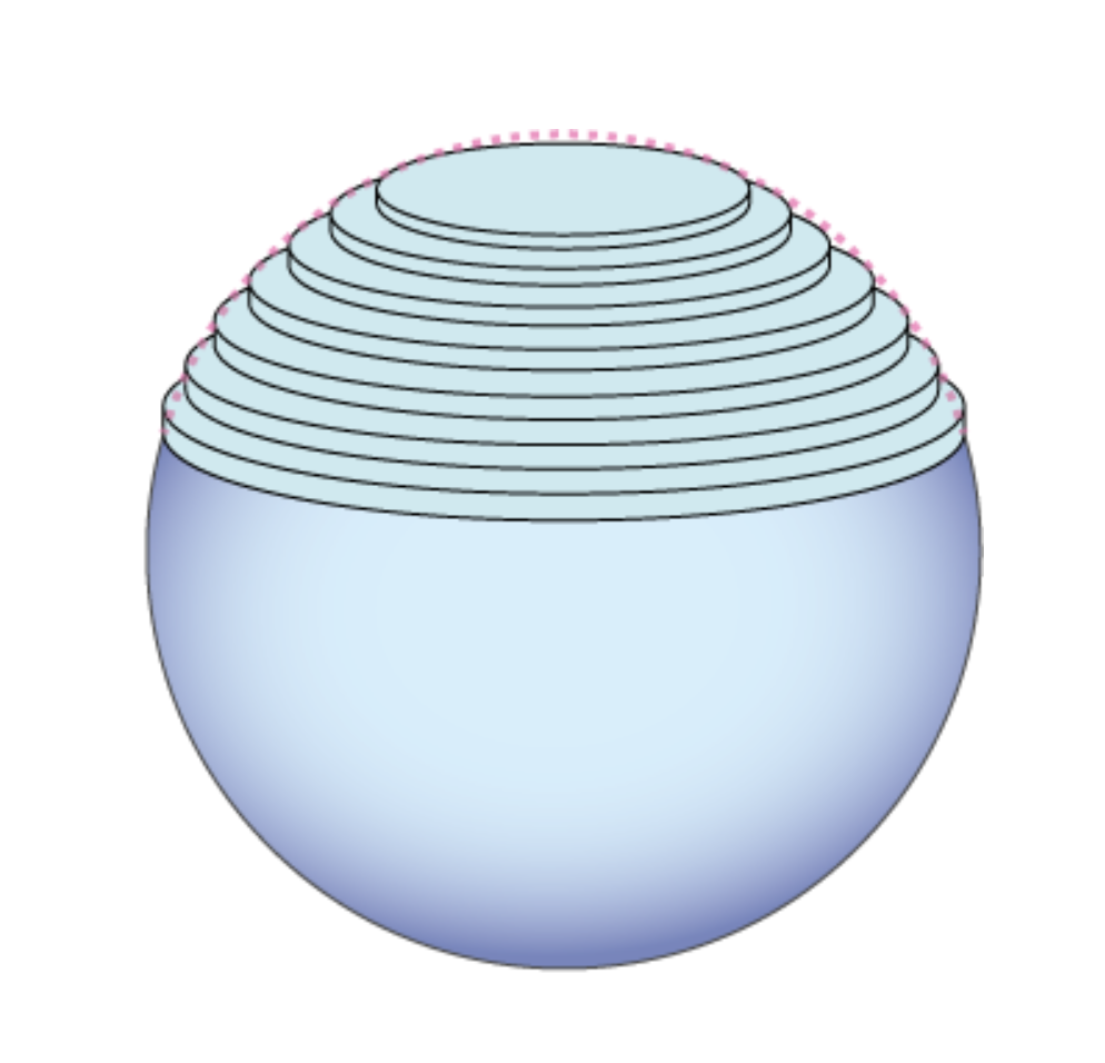
Consider an $(n+1)$-dimensional unit ball made up of $n$-dimensional disks (or balls if you will). From the definition of a unit hypersphere,

\[x^2 + y_1^2 + y_2^2 + \cdots + y_n^2 \leq 1 ,\]

we find that for fixed value of $x$, the remaining $y$-coordinates form an $n$-dimensional ball (disk when $n=2$) of radius $r(x) = \sqrt{1 - x^2}$. The volume of this $n+1$ ball is therefore just it’s lower dimensional volume integrated over the $n$ axes for $x \in [-1, 1]$:

\[V_{n+1} = \int \cdots \int_{x^2 + y_1^2 + y_2^2 + \cdots + y_n^2 \leq 1} dx \, dy_1 \, dy_2 \, \cdots \, dy_n\]

and since the integral is symmetric in every $n$,

\[= \int_{-1}^{1} V_n r(x)^n dx\] \[= V_n \int_{-1}^{1} \left( \sqrt{1 - x^2} \right)^n dx\]

If you're still wondering where that gamma function came from...

$$ = V_n \int_{0}^{1} t^{-\frac{1}{2}} (1 - t)^{\frac{n}{2}} \, dt $$ $$ = V_n \text{Beta}\left(\frac{1}{2}, \frac{n+2}{2}\right) $$ $$ = V_n \frac{\Gamma\left(\frac{1}{2}\right) \Gamma\left(\frac{n+2}{2}\right)}{\Gamma\left(\frac{n+3}{2}\right)} $$ $$ V_{n+1} = \frac{\pi^{n/2}}{\cancel{\Gamma\left(\frac{n}{2} + 1\right)}} \cdot \frac{\Gamma\left(\frac{1}{2}\right) \cancel{\Gamma\left(\frac{n+2}{2}\right)}}{\Gamma\left(\frac{n+3}{2}\right)} $$ $$ \scriptstyle{\text{where } \Gamma\left(\frac{1}{2}\right) = \sqrt{\pi}} $$ $$ = \frac{\pi^{(n+1)/2}}{\Gamma\left(\frac{(n+1)}{2}+1\right)} $$ Notice that we again assumed a unit sphere. You can show that this generalises by considering $\int_{-r}^{r} \left( \sqrt{r - x^2} \right)^n dx$ and using a nice substitution. Good luck!

Now we can see more clearly, that the dimensionality scales up the integral of a decaying function $r(x) = \sqrt{1 - x^2}$, which represents the radius of a hypersphere sitting in $n-1$. Now observe what happens to the area under $r(x)$ as we increase $n$:

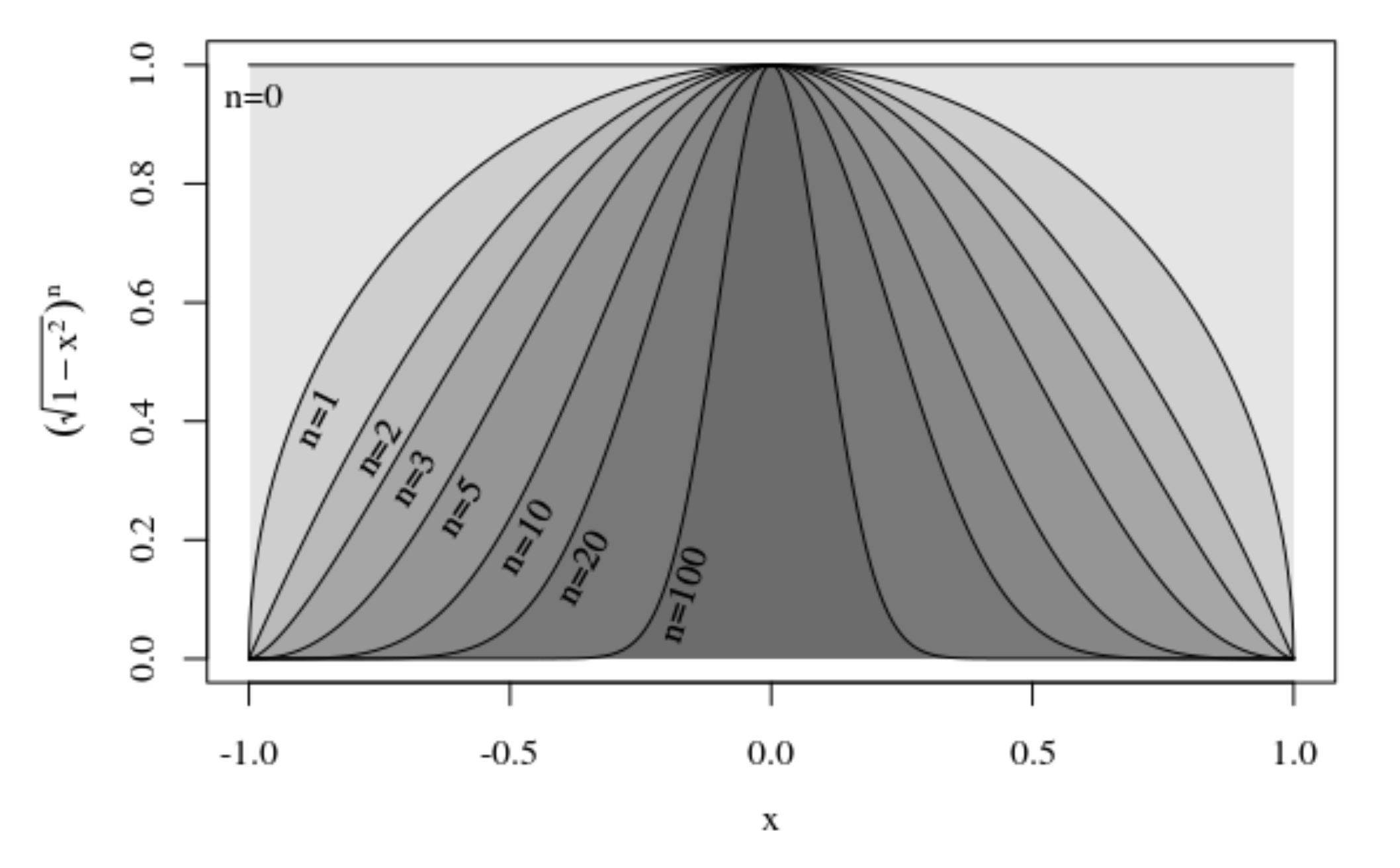
The integral collapses to zero as $n \rightarrow \infty$.

An interesting behaviour is that $r(x)$ spikes around $x=0$, and the area gets squeezed from the tails a lot more quickly than it does from the center. Remember that when $x=0$, the radius is at its maximum: $r(0) = 1$. So the integral contributes almost all of its weight around the edge of the hypersphere.

Things are slightly weirder still..

If we plot $\frac{\pi^{n/2}}{\Gamma(n/2 + 1)} r^n$, we see that the volume maximises around $n=5$, before dropping to zero.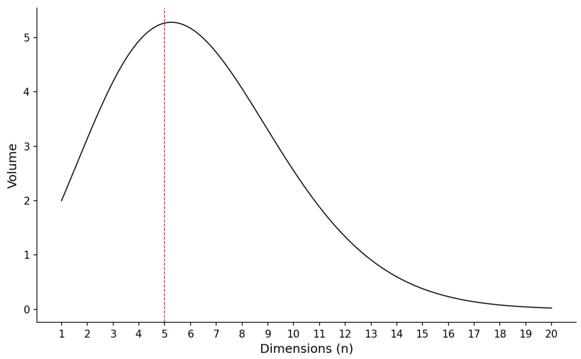

As far as I can tell, this maximum is arbitrary and has no practical implications.

---

So, in high dimensions the density is highest around the outer shell of the hypersphere. Think about what this means for sampling i.i.d. from $ \mathbf{x} = \boldsymbol{\mu} +\boldsymbol{\epsilon}$ centered on the sphere: even for small $\boldsymbol{\epsilon}$ the points will be concentrated around the outer shell. This has important implications in machine learning, contributing to what is known as the curse of dimensionality.

This phenomenon applies to other geometries too. For instance, as $n \to \infty$, the volume of a unit hypercube concentrates around a film, hugging its edges. The reason I have mentioned all of this is that these shells lead to an interesting property for high dimensional space: the average pairwise distances between points in space converges to a constant, proportional to $\mathbf{\sqrt{n}}$ – i.e. every point is equally far away from every other point. This is not intutive in our low-dimensional world.

We can see this by taking $\mathbf{x} = (x_1,\dots,x_n)$ and $\mathbf{y} = (y_1,\dots,y_n)$ as two i.i.d. points in $[-1,1]^n$, then $$ \|\mathbf{x} - \mathbf{y}\|^2 = \sum_{i=1}^n (x_i - y_i)^2. $$

$$ \mathbb{E}[(x_i - y_i)^2] = \mathbb{E}[x_i^2] + \mathbb{E}[y_i^2] - 2\mathbb{E}[x_i]\mathbb{E}[y_i]. $$ For $x_i \sim \text{Uniform}[-1,1]$, $$ \mathbb{E}[x_i] = 0, \quad \mathbb{E}[x_i^2] = \frac{1}{3} $$ Thus, $$ \mathbb{E}[(x_i - y_i)^2] = \frac{1}{3} + \frac{1}{3} - 0 = \frac{2}{3}. $$ The squared distance is the sum of $n$ independent terms, so by linearity of expectation: $$ \mathbb{E}[\|\mathbf{x} - \mathbf{y}\|^2] = n \cdot \mathbb{E}[(x_i - y_i)^2] = n \cdot \frac{2}{3}. $$ Taking the square root (approximately, as $\mathbb{E}[\sqrt{X}] \neq \sqrt{\mathbb{E}[X]}$, but grows similarly):

We find that

\[\mathbb{E}[\|\mathbf{x} - \mathbf{y}\|] \propto \sqrt{n}.\]

This concentration of measure phenomenon has important implications.

To reiterate, in high-dimensional space, most of the volume concentrates near the surface, leaving the interior sparsely populated. This leads to, on average, data points from the same distribution to being found equidistant from each other, and intuitive geometric notions, such as “closeness,” lose their meaning.

Clustering or other similarity search methods rely on relative distances so require exponentially many samples to tease out meaningful structure between data points.

---

Of course, the most interesting forms of data we encouter today (cats) rarely come from a single distribtion: they come from hierarchies of generative processes. For instance, a British shorthair might be generated from a generator of cat breeds, which in turn is generated from a feline generator, and so on. In such a hierarchical generative model, each child generator adds its own small shift (in mean and variance) relative to its parent. Notice that we use the term “generator” to emphasise an active stochastic process for creating data points that can be statistically described by “distributions”.

Let’s try and understand why this concentration of measure phenomenon is not an issue in hierarchically generated distributions:

Suppose we have two distinct generators, $\mathcal{G}_A$ and $\mathcal{G}_B$, each producing samples in $\mathbb{R}^n$. Specifically: \(\mathbf{x}_A = \boldsymbol{\mu}_A + \boldsymbol{\epsilon}_A, \quad \mathbf{x}_B = \boldsymbol{\mu}_B + \boldsymbol{\epsilon}_B,\) where $\boldsymbol{\mu}_A, \boldsymbol{\mu}_B \in \mathbb{R}^n$ are the respective mean vectors and $\boldsymbol{\epsilon}_A, \boldsymbol{\epsilon}_B$ represent i.i.d. noise with small variance (relative to the dimension $n$).

• Within‐generator distance: For two points from the same generator, say $\mathbf{x}_A, \mathbf{x}’_A \sim \mathcal{G}_A$, the vectors share the same $\boldsymbol{\mu}_A$. Their difference is mostly just $\boldsymbol{\epsilon}_A - \boldsymbol{\epsilon}’_A$, which grows on the order of $\sqrt{n}$ (by concentration of measure).

• Between‐generator distance: For a point from $\mathcal{G}_A$ and one from $\mathcal{G}_B$, the difference $\mathbf{x}_A - \mathbf{x}_B$ includes the shift $\boldsymbol{\mu}_A - \boldsymbol{\mu}_B$. Even a modest shift $|\boldsymbol{\mu}_A - \boldsymbol{\mu}_B|$ becomes amplified in high dimensions, making inter‐generator distances typically larger than intra‐generator distances.

Consequently, in large $n$, data from each generator will concentrate into distinct shells or manifolds with negligible overlap. Sibling generators (e.g. two cat breeds) form shells far apart from one another, yet each remains close within its own breed’s shell. Child shells nest inside or near the parent shell (all domestic cats remain within the broader feline shell), but are still distinct from other child shells at the same level. This “push” into separate shells is not something we exploit in low dimensions—but it emerges naturally in high dimensions, giving us surprisingly clear separations between different concepts. In deep learning, one can think of hidden‐layer representations as “discovering” or approximating these shells.

---

So in the end, the curse of dimensionality is a double-edged sword:

Curse: For single high‐dimensional distributions, pairwise distances become uniform and clustering methods fail without exponentially more data.

Blessing: Once you have hierarchically generated distributions, high dimensionality amplifies even small differences among them, yielding distinct shells that are easier to separate. Points in the same shell stay “close”, even though the space becomes exponentially large.